Chess as autocomplete
Can autocomplete play chess blindfolded? A journey into applied AI research
Play against the final model directly in your browser.
A 91M parameter transformer sees only chess moves (plus three tokens naming the players' ratings and the time control), never the board, never the rules. It learns to play blindfolded at near-state-of-the-art human move accuracy, purely by getting good at predicting the next token.
In my previous article, we built a mental model of LLMs as autocomplete.
As a quick recap: LLMs are given the sentence
and simply predict the next token.
So in theory, if we frame the game of chess as a language autocomplete problem, we should be able to train an LLM to play chess.
Can we train a transformer to play chess blindfolded by autocompleting the language of chess?
Blindfold chess is a variant of chess where the players do not see the board. Someone reads out the moves to them, and they reply by announcing their own next move out loud.
This sounds exactly like the framing we want: moves in, moves out.
The most commonly used language to represent chess games is called Standard Algebraic Notation (SAN). For example, the Italian Game starts with the moves
1. e4 e5 2. Nf3 Nc6 3. Bc4
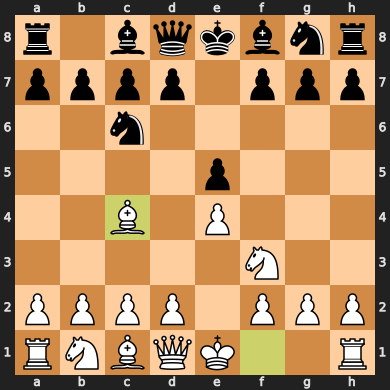
And can be understood as follows:
| White | Black | |
|---|---|---|
| 1. | e4♙︎ pawn e2 → e4 | e5♟︎ pawn e7 → e5 |
| 2. | Nf3♘︎ knight g1 → f3 | Nc6♞︎ knight b8 → c6 |
| 3. | Bc4♗︎ bishop f1 → c4 |
If you wish to explore SAN in detail you can go to this chess.com article.
Why and what?
…general methods that leverage computation are ultimately the most effective, and by a large margin.
Richard Sutton, The Bitter Lesson, 2019
This project takes that idea to an extreme. Karvonen (2024) showed that a small GPT trained on move text alone learns the board well enough to be probed for it, at 16 million games and 25M parameters. As far as I know nobody has run that idea at scale: a general model (a standard model with nothing chess-specific added: no board, no search, no extra heads) trained on a massive corpus of human games. One transformer, trained on nearly 1.8 billion human games, about a hundred times that corpus.
Predicting the next move in a game is the same problem an LLM solves predicting the next word, so I borrow the whole apparatus: a decoder-only transformer (the model family behind ChatGPT) trained with the recipe modern LLMs are built with. The interface is tokens in, tokens out, nothing else: the model only ever sees a stream of moves and learns to continue it.
The model must learn to calculate everything else: where every piece sits, whose turn it is, which moves are even legal. It reconstructs all of it from the move stream alone. That is blindfold chess in the most literal sense.
Deep diveHow others teach models to play chess like humans
Plenty of others have taught machines human-like chess. They differ in how much chess is built into the architecture, whether they search at move time, whether they learn from a strong engine like Stockfish, and how much data they train on. This project sits at the spare end of the first three (no board, no search, no engine teacher) and leans on the last: data.
| System (year) | Chess-specific architecture | Search / engine teacher | Training positions | Params | Time controls |
|---|---|---|---|---|---|
| Maia (2020) | 8×8 board planes; AlphaZero-style CNN; last 12 plies fed in | None | ≈0.6B 1 | 10.3M (×9) | Blitz/rapid/classical |
| Maia-2 (2024) | Board planes; ResNet CNN + skill-aware attention | None | 9.1B | 23.3M | Rapid only |
| Maia-3 / Chessformer (2026) | 64 squares as tokens; geometric attention bias; policy + value heads | None | ≈0.5B 2 | 79M | Blitz only |
| Grandmaster without search (2024) | FEN snapshot tokenized; action-value classification head | Stockfish teacher | ≈0.53B 3 | 270M | n/a |
| Allie (2024) | Decoder-only LM over UCI move tokens; + value & think-time heads | MCTS search | ≈262B 4 | 355M | Blitz only |
| This post | None: vanilla decoder-only LM over move tokens; no board, no value head | None | 122.9B | 91M | All four |
Position = one board state trained on; one move token per ply for the move-stream LMs (Allie, this post). Time controls = the Lichess game speeds in the training data; "all four" = bullet, blitz, rapid, classical.
- Maia: ≈0.6B per model, one per rating bin (×9); 12M games/model × ~50 kept moves/game; model sees 409.6M (400k steps × 1024 batch).
- Maia-3: corpus size unpublished; ≈512M positions processed in training (1M steps × 512 effective batch), shown as a scale proxy.
- Grandmaster: 15.3B Stockfish action-value labels over ≈0.53B distinct positions.
- Allie: 6.6B-token training set (91M games) trained ~40 epochs (2M steps × 131,072 tokens), so ≈262B tokens seen; the 6.6B is the dataset, the 262B the total seen during training.
Board-based human imitators: the Maia line. Maia (McIlroy-Young et al., 2020) reframed the goal of chess AI from playing the best move to predicting the move a human of a given rating would actually play. It uses an AlphaZero-style convolutional network that reads the board as a stack of 8×8 planes (so the board, its geometry, and the legal moves are built in rather than learned), and it plays with no search. The catch is that "a given rating" meant nine separate models, one per 100-Elo band. Maia-2 (Tang et al., 2024) folded those into one network with a "skill-aware attention" module that conditions on both players' ratings, and Maia-3 / Chessformer (Monroe et al., 2026) pushed the idea furthest: a transformer that still reads the board, now as 64 square-tokens with a learned geometric attention bias, and currently holds the human move match record among board-based models (57.1% at 79M parameters).
The engine-distillation outlier. DeepMind's Grandmaster-Level Chess Without Search (Ruoss et al., 2024) is the odd one out. It is also a searchless transformer, but it does not learn from humans at all: it reads a board (a tokenized FEN) and is trained to reproduce Stockfish 16's win probability for every legal move, on the order of 15 billion engine evaluations, with human games used only as a source of positions. The result plays at grandmaster strength (~2895 Lichess blitz Elo) without ever searching. It distills an engine rather than imitating people; its goal is strength, not human-likeness.
The world-model probes: Chess-GPT. Adam Karvonen (2024) trained small GPTs on nothing but PGN text, character by character, then went looking inside them. Linear probes recover the state of every square to 99.6% accuracy: a model given no board builds one anyway. A second probe separates players below 1550 Elo from those above 2050 with 90.5% accuracy, so the model estimates skill as a latent variable purely to predict the next character better, which is the unsupervised version of the metadata tokens this project feeds in explicitly. It is the chess version of the Othello-GPT result. What differs here is scale: 16 million games at 25M to 50M parameters, against 1.76 billion games. Karvonen establishes that the effect exists; this post asks what it is worth when the corpus is a hundred times larger and the model is trained to be played rather than probed.
The move-stream cousin: Allie. Allie (Zhang et al., 2024) is the closest relative to this project: a decoder-only transformer over a stream of moves (in UCI notation), a language model of chess in the same sense ours is. It trains "exclusively from humans" (no engine distillation) and adds heads that predict how long a human would think and how the game will end. Its search-free policy scores 55.7% move match, in the same range this project lands in. The headline difference is its "bit of search": a Monte-Carlo tree search whose budget scales with the model's own predicted human think-time. That search keeps Allie calibrated against very strong opponents; this project, with no search at all, gives that up.
Every time control, not one. The human imitators here each train on a single slice of Lichess: Maia-2 on rapid, Maia-3 and Allie on blitz, and even the original Maia throws out bullet. Fast games get dismissed as noise, classical as too scarce. We train on all time controls.
Where the others add a board, a search, an engine teacher, or extra heads, this one adds only data: a single pass across every time control rather than many passes over a narrow slice. That is what makes it a general model in the sense above, rather than a chess-specific one.
Hardware and compute
This being a personal project, I do not have access to large computational resources. I have a personal computer with an Intel i5-13500 CPU, an NVIDIA RTX 4070 Ti Super (16 GB) GPU, 16 GB of RAM, and under 1 TB of available storage. This will impact several engineering choices made throughout the project. Partway through the project I unexpectedly gained access to a couple of VMs with A100 and H100 GPUs, but by then those choices had already been shaped by the hardware above.
Pre-training
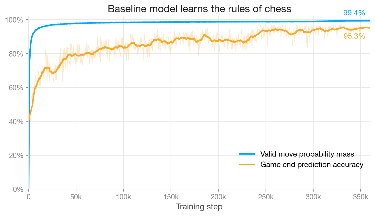
The goal of pre-training our chess autocomplete is to learn the language of chess, the rules of the game. We will measure the performance of a pre-trained model with two metrics:
- Valid move probability mass (VPM): the sum of the probabilities the model assigns to all legal moves in a position, averaged over all positions. In plain terms: what fraction of the model's probability lands on moves that are actually legal. A legal move in this definition includes a piece move or a valid draw claim (threefold repetition). Predicting a terminal state like checkmate incorrectly is also considered an invalid move. A model that has fully learned the rules would score 100%.
- Game-end prediction accuracy (GPA): measures the accuracy of the model when predicting how a game ended (checkmate, stalemate, draw by repetition, fifty move rule). How often does the model correctly predict when and how the game ends.
For move validity, the important number is the valid move probability mass and not the top-1-legal rate. This is because we may sample from the output distribution to choose the next move, and this metric correctly shows the probability of sampling an illegal move.
For game end prediction however, the correct metric is how often the most likely output is the correct game end prediction. Whenever the model output is a game end prediction, we never sample; we always pick the most likely one. That is why accuracy is the right metric here, not probability mass.
These two metrics will give us a way to evaluate how well the model has learned the rules of chess. Our goal is to reach 100% VPM and 100% GPA.
We will also get a sense of the model's playing strength by playing it against the Stockfish 18 chess engine at a range of strength levels. This is not an explicit optimization target: the goal of this project is not to build the highest-rated chess model, only to understand how well a model trained as pure autocomplete ends up playing.
The dataset
The open-source online platform Lichess publishes the games played on their platform as an open database. This database contains (as of May 2026) a total of 7,863,012,346 rated chess games, spanning over 13 years, from complete beginners to grandmasters. This database has a total compressed size of 2.49 TB.
Elo peaks at around 1500, which may be because players start with 1500 Elo on Lichess. The most popular time controls are blitz and bullet, followed by rapid, ultrabullet, and classical.
Deep diveFrom 7.8 billion games to a training set
The Lichess open database holds about 7.8 billion games, but the final model never sees most of them. It trains on the 21 monthly standard-rated files spanning January 2024 through September 2025, 1,950,403,943 games. The validation set is held out as the most recent 10% of games from the newest file (September 2025); everything before that is training data.
The files are read newest first, and the 600,000-step budget runs out before the pool does. The run ends 13% into the February 2024 file and never opens January 2024, so it sees 1.76 billion of those games, 90% of the pool, almost all of them exactly once.
Lichess implements a couple of rules differently than other platforms. A threefold repetition is not an automatic draw: the side to move has to claim it, and many players simply play on, so the data routinely holds positions sitting on a repetition nobody claimed (Lichess only forces the draw on the fifth repetition). The fifty move rule is the opposite: Lichess draws the game automatically the moment it applies, so no game ever continues past it.
Data processing
The games in the Lichess open database are stored as zstd compressed PGN (portable game notation) files. A PGN file is a commonly used text format for storing both metadata and moves from one or more games of chess. Below is an example of the PGN of a chess game.
[Event "Troll Masters"]
[Site "Gausdal NOR"]
[Date "2001.01.05"]
[Round "1"]
[White "Edvardsen,R"]
[Black "Carlsen,Magnus"]
[Result "1/2-1/2"]
[WhiteElo "2055"]
[BlackElo ""]
[ECO "D12"]

1.d4 Nf6 2.Nf3 d5 3.e3 Bf5 4.c4 c6 5.Nc3 e6 6.Bd3 Bxd3 7.Qxd3 Nbd7 8.b3 Bd6
9.O-O O-O 10.Bb2 Qe7 11.Rad1 Rad8 12.Rfe1 dxc4 13.bxc4 e5 14.dxe5 Nxe5 15.Nxe5 Bxe5
16.Qe2 Rxd1 17.Rxd1 Rd8 18.Rxd8+ Qxd8 19.Qd1 Qxd1+ 20.Nxd1 Bxb2 21.Nxb2 b5
22.f3 Kf8 23.Kf2 Ke7  1/2-1/2
The moves in a PGN file are stored in SAN. SAN is convenient for chess players, but it is not the most convenient representation for this project, for reasons we get into when choosing the model's input representation.
Binary game representation
I designed a compact 16-bit binary format: every move fits in exactly two bytes, can be decoded on its own without replaying the game, and any game can be read straight out of the middle of a file. The full bit layout (and the two companion files that make individual games randomly addressable) are in the deep-dive below.
Deep diveDataset representation
To give a sense of scale: our complete training set, the 21 monthly Lichess files from January 2024 through September 2025, is 635 GB compressed and about 4.2 TB uncompressed as PGN. In our binary representation it takes only 292 GB, itself uncompressed and supporting O(1) random access to any game.
Encoding one PGN file produces a triplet of files that share a base name. For the September 2025 database that is:
…2025-09.bin: the moves of every game, back to back.…2025-09-map.bin: one byte offset per game, for random access.…2025-09-metadata.parquet: one row of metadata per game.
The three files are aligned by row index: game N in the .bin is entry N in the map and row N in the parquet.
The moves: .bin
The move format was designed against these requirements:
- Contains all necessary information
- Which piece was moved
- From which square
- To which square
- If it was a promotion, to which piece
- If it was a castling move, which one
- If the game ended, how
- Can be quickly parsed without a board representation
- Byte aligned
- As space efficient as possible
- Allow random access to games
- No lookup tables
The sixteen bits are laid out as five fields: a move type, then the from-square and to-square as file/rank pairs:
The first 4 bits encode the move type:
| Bits | Move type | Bits | Move type |
|---|---|---|---|
0000 | Pawn move | 1000 | Game end |
0001 | Knight move | 1001 | Promotion to knight |
0010 | Bishop move | 1010 | Promotion to bishop |
0011 | Rook move | 1011 | Promotion to rook |
0100 | Queen move | 1100 | Promotion to queen |
0101 | King move | 1101 | Black king side castle |
0110 | White king side castle | 1110 | Black queen side castle |
0111 | White queen side castle | 1111 | Unused |
The remaining 12 bits encode the from-square and to-square as two file/rank pairs of 3 bits each:
| Bits | File | Rank |
|---|---|---|
000 | a | 1 |
001 | b | 2 |
010 | c | 3 |
011 | d | 4 |
100 | e | 5 |
101 | f | 6 |
110 | g | 7 |
111 | h | 8 |
En passant needs no special move type: it is stored as an ordinary pawn capture. The 16 bits alone do not reveal that the captured pawn sits on a different square than the destination, but that is recoverable from the position, and nothing in the pipeline needs it.
And there are 6 "special" numbers representing game end states:
| Token | Value | Meaning |
|---|---|---|
<|unknown|> | 0x8000 | Recorded moves run out before any real ending |
<|checkmate|> | 0x8001 | Checkmate |
<|stalemate|> | 0x8002 | Stalemate |
<|insufficient_material|> | 0x8003 | Insufficient material |
<|fifty_move_rule|> | 0x8004 | Fifty-move rule |
<|threefold_repetition|> | 0x8005 | Threefold repetition |
Each game is its move tokens followed by exactly one of these end tokens, and games are written one after another with no separator between them: the end token doubles as the boundary. Every token is two bytes, little-endian, so the file is exactly two bytes per token from start to finish. Every special token (the six endings and <|game_start|>) uses move-type 1000, a code no real move occupies, so it can never collide with a move.
Random access: -map.bin
Scanning for end tokens walks the file front to back, but jumping straight to game five million needs an index. The map file is a flat array of uint64 little-endian byte offsets, one per game, each holding the end byte position of its game in the .bin. Game 0 starts at byte 0 and game i starts where game i-1 ended, so two adjacent entries bracket any game in constant time. The training pipeline memory-maps both files and reads a game as a single slice.
Who was playing: -metadata.parquet
The .bin deliberately holds only moves; everything about a game lives in a separate parquet file, one row per game in the same order. Keeping it apart leaves the moves a clean token stream, and lets anyone filter the dataset on metadata without touching the binary. The columns:
| Column | Type | Meaning |
|---|---|---|
GameIndex | u64 | 1-based position of the game in the source PGN, counting games later skipped |
WhiteRating/16 | u8 | White Elo divided by 16 |
BlackRating/16 | u8 | Black Elo divided by 16 |
InitialTime | u16 | Initial clock, in seconds |
Increment | u8 | Increment per move, in seconds |
GameIndex counts the skipped games too, so any row traces back to its exact game in the original PGN.
The September 2025 Lichess open database file has a total of 87,049,890 games, a compressed size of 28.3 GB, and an uncompressed size of about 189 GB. Encoding it produces an 11 GB .bin, a 0.7 GB map, and a 0.5 GB metadata file, about 12.5 GB in total. This is about a 15x reduction from the uncompressed size, and 2x reduction from the compressed size.
A baseline, we have to start somewhere
The initial goal is to see whether this can work at all. I designed a simple transformer, a simple tokenization strategy and a simple training procedure.
Choosing an input representation for the transformer
The most obvious representation would be to use SAN directly: map every possible SAN move to its own token. I discarded this early, for two reasons.
First, SAN is not self-contained. A move like Nxf4 tells you a knight captured on f4, but not which knight or from where; to recover that you have to replay the game on a board. I wanted a representation that makes the piece, the from-square and the to-square explicit, keeping our options open for the rest of the project.
Second, the same physical move can be written several different ways depending on what else is on the board, and if it gives check, a + is appended, adding yet another spelling like Nxf4+. Mapping SAN straight to tokens would force the model to learn a separate token for each spelling, although they all mean the same move:
- Nxf4only one knight can reach f4
- N5xf4a second knight on d3: same file, disambiguate by rank
- Ndxf4a second knight on h5: same rank, disambiguate by file
For simplicity's sake I opted to start by using our 16-bit binary game representation, where each of the 2^16 possible moves represents its own token. This also comes with the added benefit of not needing a tokenizer, since the binary move representations are our tokens. We only need to add a <|game_start|> token.
A tokenized game ready to be processed by our model looks like:
The model never receives <|unknown|> as a target. This is because <|unknown|> can mean that a player resigned, a draw was agreed, a player timed out, etc. We do not want the model to predict any of these. Who wants a chess engine that resigns?
Model definition and training (v0)
I opted to start with a simple decoder only transformer following the same architecture as GPT-2 with the same hyperparameters as the smallest GPT-2 model with some minor modifications. The model is trained on the first 64 half moves (plies) of each game, for a total of 360k steps: 138 million games, 8.8 billion tokens, 36.7 hours of training.
Deep diveModel and training configuration
- dimension
- 768
- num heads
- 12
- num blocks
- 12
- positional encoding
- RoPE
- non-linearity
- GELU
- vocabulary size
- 216
- max sequence length
- 64
- batch size
- 384
- optimizer
- AdamW (weight decay 0)
- max learning rate
- 6e-4
The model is trained on a max sequence length of 64 (64 half moves) for a total of 360k steps (138.2 million games). The learning rate is kept at 6e-4 for the first 300k steps, and then decayed to zero over the next 60k steps following an inverse square root schedule.
At the end of the 360k steps the model reached 99.4% VPM and 95.3% GPA on the validation set:
Playing strength over 100 games per opponent, scored as an Elo performance rating (the Elo you would need to score that result against that opponent):
| Opponent | Win | Draw | Loss | Performance rating |
|---|---|---|---|---|
| Stockfish, 1347 rated | 61.0% | 9.7% | 29.3% | 1464 |
| Stockfish, 1566 rated | 37.1% | 11.8% | 51.1% | 1516 |
A rating around 1490. The language of chess has been learned, mostly. Now to improve on it.
Improving the baseline model
The baseline gave us a working training pipeline and several places to improve it. I followed the process of creating hypotheses of what could improve the model, then testing these hypotheses with real training runs. Testing different configurations one by one and evaluating their performance is referred to as an ablation sweep. Below are the improvements made.
Deep diveHow the sweep was run
The sweep rests on one number: the noise floor. The baseline configuration was trained five times with different random seeds, and the seed-to-seed standard deviation of the validation loss came out at 0.0038 nats (a nat is just the natural-log unit the loss is measured in). That sets the bar for what counts as a real change rather than luck.
- One change at a time, equal compute. Every run gets the same budget of 7.93x10¹⁷ FLOPs (floating-point operations, a hardware-independent measure of how much computation a run costs), about 1.5B tokens, roughly one hour on the Azure H100. This is the “small” budget.
- A two-sigma gate. A change is accepted only if it beats the baseline by more than two standard deviations, 0.0077 nats. Anything inside that band is noise, no matter how promising it looks.
- Survive scale. The best variants are re-run at 4x the compute with three seeds each, to check the win does not evaporate once the model trains longer. Several did not survive it.
In total the sweep took 47 training runs and about 123B training tokens, almost exactly what the single final run would later consume on its own.
A vocabulary of impossible moves
Our binary representation gives us 65,536 possible tokens, but the vast majority of them are moves that can never be played: a pawn moving from a1 to h8, a king jumping across the entire board, a rook moving diagonally. If we only keep the moves that can actually occur on a chess board we are left with 4,128 tokens. I call this the realizable vocabulary.
Switching the input to the realizable vocabulary reduced the number of parameters from 186M to 138M. Switching the output to this vocabulary further reduced the number of parameters down to 91M. Over half of the baseline model was spent embedding/decoding tokens that can never appear in a game.
The sweep confirmed it. The realizable input/output combination was the best of every encoder/decoder tested.
Deep diveHow 65,536 moves become 4,135
The realizable vocabulary is built by enumerating every move that is geometrically possible on an empty board, for every piece type and every square:
- Sliding pieces (queen, rook, bishop) along every ray out to the edge of the board.
- King and knight moves from every square.
- Pawn single pushes, double pushes, diagonal captures, and promotions, for both colors.
- The four castling moves.
That yields 4,128 distinct move tokens. Seven more describe the game rather than a move, one for the start and six for the ways a game can end, which makes the 4,135 classes the model predicts. The input side carries 36 metadata tokens on top of those: 30 rating buckets and a marker for a missing rating, then five time controls. So 4,171 tokens go in and 4,135 come out, because the model reads metadata but never has to write it. Each of the remaining ~61,000 of the 65,536 possible 16-bit words (a bishop moving like a rook, a pawn teleporting across the board) describes something that can never legally happen, so it never needs a token.
Training on full games
The initial model was trained on the first 64 half moves of each game. We consider full games to be up to 200 half moves as the vast majority of games in the dataset are finished long before that. Real games vary a lot in length, so the pipeline has to handle variable-length sequences without wasting compute on padding. The approach I chose packs games of different lengths into a single padding-free stream, so every position the GPU touches is a real move (the mechanics are in the deep dive below). This change never entered the sweep: seeing whole games is a prerequisite for learning full games, not a tuning knob to validate.
Deep diveHow games of different lengths share a batch
The simplest way to put games of different lengths in one batch is to pick a fixed width and pad. Every game becomes a row of the same length; any game shorter than that width is filled out with a padding token, and the loss is told to ignore those positions. It trains correctly, but the padding still flows through every attention and feed-forward layer. The GPU does the work and then throws it away. At a width of 64 half moves that overhead is tolerable. At 200 it is not: most games finish long before 200 half moves, so a fixed-width batch would be mostly padding, and most of the compute would go to waste.
So the batch dimension is dropped entirely. Instead of a rectangle of games, the games are concatenated into a single long stream, sized to a fixed token budget: every position in it is a real move, and there is nothing to pad. Because each step processes the same number of tokens, memory and step time stay flat from batch to batch. (The one game that would spill past the budget is cropped to fit, which costs about a hundred tokens per batch, a rounding error.)
This packing must be handled carefully: run attention naïvely over the stream and the transformer can attend across games, not good. Preventing it takes two pieces of bookkeeping. The first records where each game starts and ends, so attention can be confined to a block-diagonal pattern: every token attends only within its own game, never across a boundary. The second gives each token its position within its own game, resetting to zero at every boundary, so the rotary positional encoding numbers each game from its first move wherever it lands in the stream.
cu_seqlens marks those boundaries so attention never crosses them.In the first example, padding spends 24 tokens of compute to process 16 tokens of information; packed, the same three games take exactly 16. A third of the padded batch was wasted work.
This packed attention is implemented in FlashAttention's variable-length kernel, flash_attn_varlen_func. The ordinary kernel expects a (batch, seq_len, heads, dim) rectangle; the varlen one expects the flat stream and is told the seams. Its parameters:
flash_attn_varlen_func(
    q, k, v,
    cu_seqlens_q,
    cu_seqlens_k,
    max_seqlen_q,
    max_seqlen_k,
    causal=True,
)q,k,v: query, key and value for every token in the packed stream, shape(total_tokens, n_heads, head_dim), no batch dimension.cu_seqlens_q,cu_seqlens_k: cumulative sequence lengths, the offsets[0, 6, 9, 16]from the diagram marking where each game begins and ends. Query side and key side are the same tensor, because a token's queries and the keys it may attend to live in the same game. These seams are what make attention block-diagonal.max_seqlen_q,max_seqlen_k: length of the longest game in the batch. The kernel needs an upper bound up front to size the work it launches; it changes how the work is tiled, not the result.causal=True: inside each game a move attends only to the moves before it. Together withcu_seqlens, every token sees exactly its own game's past and nothing else.
Adding game metadata
A game between two 800 rated players looks very different from a game between two grandmasters, and the same player plays very differently in bullet than in classical. Our initial model sees none of this. It sees only moves.
The PGN headers already contain the ratings of both players and the time control, so we can give them to the model. Three metadata tokens are prepended to every game: the time control, the white player's rating, and the black player's rating. These are ordinary special tokens, the same device every LLM already uses for markers like start-of-text; the model reads them exactly as it reads a move, and nothing about the architecture changes.
But at inference time we may not know these values. To handle this, each metadata token is randomly replaced with a special token 30% of the time during training. The model learns to use the metadata when it is available, and to fall back to a sensible average when it is not.
Verdict: Metadata is a real win: given the ratings and time control, the model beats the no-metadata baseline. The dropout is what makes it safe: without it, the model falls apart whenever a value is missing.
Deep diveHow the metadata tokens are built
Ratings are not stored exactly. Each one is rounded into one of 16 buckets, 100 points wide, from 1000 to 2500; anything below 1000 lands in the bottom bucket and anything above 2500 in the top one. A 2480 and a 2530 player both become the same 2500 token.
The three tokens are always written in the order time control, white rating, black rating, immediately before <|game_start|>. The time control is one of four values: bullet, blitz, rapid, or classical.
During training, each of the three tokens is independently swapped for a token 30% of the time. That is why the model still plays when you tell it nothing: it has seen plenty of games where the rating or time control was absent. The metadata positions are never used as prediction targets: the model reads them, it never has to generate them.
A better optimizer
The baseline used AdamW for every parameter. The biggest single win of the whole sweep came from replacing it on the transformer-block weights with the Muon optimizer, while AdamW keeps the embeddings, the output layer and the norms. (The optimizer is the algorithm that turns each batch's gradients into an actual weight update.)
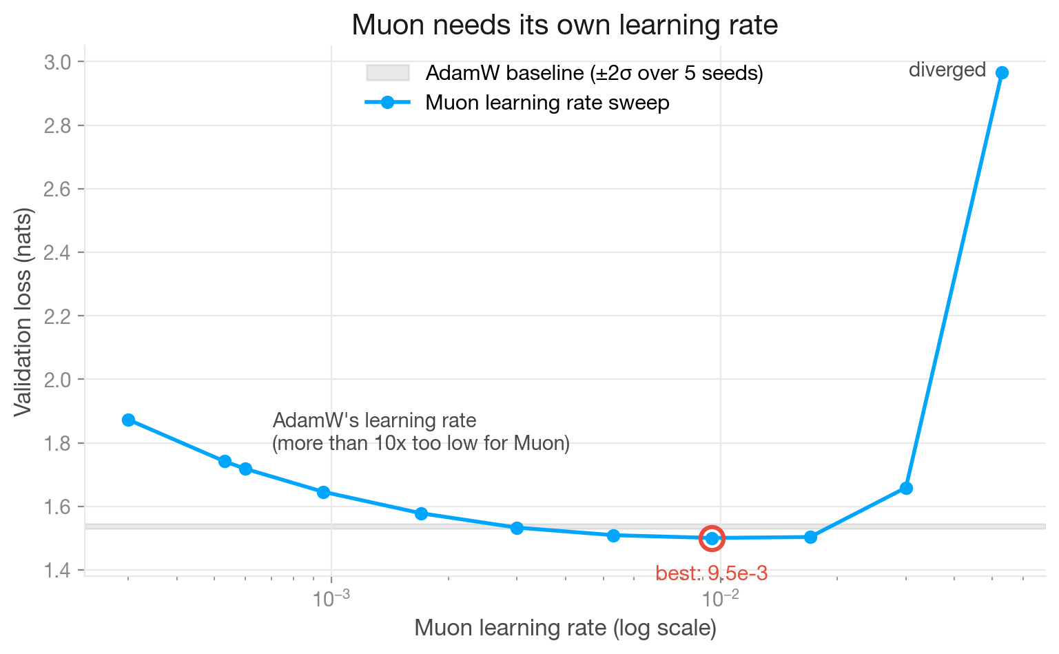
The first attempt was a disaster: reusing AdamW's learning rate of 6e-4 for Muon left the model about 0.18 nats worse than baseline. Muon wants its own learning rate, more than 10x higher. Unsurprising in hindsight, since Muon orthogonalizes its updates, so its learning rate lives on a different scale. After a proper sweep the best value was 9.5e-3. With Muon carrying the block weights, AdamW's learning rate for the remaining parameters was swept again and also preferred to be higher, landing at 1.9e-3.
Other changes that were considered but not accepted
Most of the architecture knobs turned out not to matter. A deeper, thinner model was clearly worse. A version with more attention heads never separated from baseline either way, so it was dropped without a 4x rerun. A wider, shallower one looked like a tie at the small budget and then lost outright when re-run at 4x compute, as did a higher AdamW learning rate I would otherwise have shipped. RMSNorm landed within noise of LayerNorm, so LayerNorm stays. Two parts of the final recipe rode in without an ablation win: SwiGLU (a now-standard variant of the transformer's feed-forward layer, adopted by convention because it is what modern LLMs use) and the learning-rate schedule, a constant rate with an inverse-square-root warmdown, carried over unchanged from the paper it comes from rather than tuned here. And weight decay bought nothing at this scale, so the recipe inherited none, a choice that caused problems at full scale.
Deep diveThe sweep, phase by phase
Every phase below changes one thing against the same baseline and is judged against the same gate: beat the baseline by more than 0.0077 nats (two standard deviations) to count, then get re-run at 4x compute to prove the win survives. The phases ran in roughly this order, each locking its winner before the next began.
Tokenizer and representation. The first question was how to encode a move. Feeding the model realizable tokens on the input was the best encoder of everything tested (1.531 nats vs the 1.537 baseline) and, as a bonus, dropped the ~50M-parameter input embedding for free. The decisive result was on the output side: keeping the full 65,536-token output layer was catastrophic, around +0.06 nats worse at equal compute and down on every auxiliary metric.
Metadata tokens. Prepending the ratings and time control is a clear win when the model is given them (about -0.017 nats) but the interesting question was what happens when it is not. A model trained with no dropout on the metadata learns to lean on it so hard that, asked to play without it, it falls apart: +0.23 nats worse than its own with-metadata score, well below even a model that never saw metadata. Training with 30% dropout removes the dependence: without metadata, it sits right on the no-metadata baseline; with metadata, it keeps almost the whole win. That is the variant in the recipe.
Optimizer sanity check. Before tuning anything exotic, I checked the optimizer settings inherited from modded-nanogpt: the AdamW betas, and weight decay. Nothing beat the gate. Notably, adding the standard weight decay of 0.1 was a no-op at this scale (it bought nothing), so the recipe kept weight decay at zero. That looked safe here. It was not safe at 20x the compute.
Model shape. Holding the parameter count roughly fixed, I tried trading width for depth. A deeper, thinner model (576-wide, 21 blocks) was clearly worse, +0.019 nats. A wider, shallower one (1024-wide, 7 blocks) and a version with twice the attention heads were both statistical ties, and the wider one trained about 20% faster, which made it tempting. It was promoted to the 4x round, where the tie broke against it.
Learning rate, before Muon. Sweeping AdamW's learning rate a half-decade each way around the inherited 6e-4 showed 6e-4 was conservative: 1e-3 won by -0.014 nats at the small budget. Going the other way fell off a cliff: 3e-4 and below collapsed entirely. So 1e-3 was promoted to the 4x round. Like the wide-shallow shape, it then failed to hold up.
Normalization and the MLP. RMSNorm, the now-common alternative to LayerNorm, was run at 4x compute and landed +0.0015 nats from LayerNorm, inside the noise band, on the wrong side of zero. The MLP never got that treatment. A SwiGLU ablation was written and staged, then never run at any budget, and SwiGLU went into the final recipe anyway on the strength of what modern LLMs do. The other untested choice is the learning-rate schedule: the constant-then-inverse-sqrt warmdown was carried over unchanged from the paper it comes from and never ablated.
Muon optimizer. The largest result in the sweep was switching the transformer-block weights to Muon. The first run buried it: handed AdamW's 6e-4, Muon came out +0.18 nats worse than baseline, and a naïve reading would have thrown the optimizer out. Sweeping its learning rate across a log grid told the real story: Muon wants roughly 10–15x AdamW's rate, with a broad good valley from about 5e-3 to 2e-2 and a hard divergence cliff past it (5.3e-2 blew up entirely). The best point, 9.5e-3, beat the baseline by -0.036 nats, by far the biggest single win. Best-case Muon also beat best-case plain AdamW by another -0.022.
AdamW's rate, with Muon locked in. With Muon carrying the block weights, the remaining AdamW parameters (embeddings, output layer, norms) got their own learning-rate sweep. It improved monotonically up to 1.9e-3 with no cliff in the tested range, so that is the value used, though the gain over the previous setting is inside the noise gate: the best observed point rather than a proven optimum.
Surviving 4x compute. The whole point of the final round was to keep the small-budget winners honest. Two of them did not make it: the wider-shallower shape and the higher AdamW learning rate both shed their edge once the models trained four times as long, ending up clearly behind the plain choice. The realizable tokenizer, the original shape, and the metadata-with-dropout win all held (metadata stayed about -0.015 nats ahead at scale, and free in the worst case) and those are what went into the final recipe.
The final model
With the ablation sweep finished, every choice is settled. The final recipe:
- dimension
- 768
- num blocks
- 12
- num heads
- 12
- normalization
- LayerNorm
- non-linearity
- SwiGLU
- parameters
- 91M
- input vocab
- 4,171
- output vocab
- 4,135
- metadata dropout
- 30%
- Muon lr (blocks)
- 9.5e-3
- AdamW lr (rest)
- 1.9e-3
The final training run takes this recipe to the full training set: 600,000 steps, about 123B tokens of chess games (600,000 steps × 1,024 sequences × 200 half moves), a single near-complete pass in which almost every game is seen exactly once. It did not go smoothly the first time (the first attempt exploded past step 160,000 and had to be restarted with a small amount of weight decay added) but the rerun trained cleanly all the way through, three and a half days on the H100. The result is chess-autocomplete-v1-91m, the model you can play against at the top of this page.
- max sequence length
- 200
- batch size
- 1,024 (512 microbatch × 2 accumulation)
- steps
- 600,000
- weight decay
- 0.01 Muon / 0.005 AdamW
- schedule
- constant, then inverse-sqrt warmdown over the last 120k steps
Deep diveThe final run
The recipe that came out of the sweep carried no weight decay, and the first attempt at the final run did not survive that. At step 160k everything was healthy: validation loss falling, VPM at 100%, gradient norms (the overall size of each update step) around 0.08. At step 165k the gradient norm spiked to 55. By step 172k it had reached 108. The validation loss climbed to 23.8, and VPM collapsed to 1.8%.
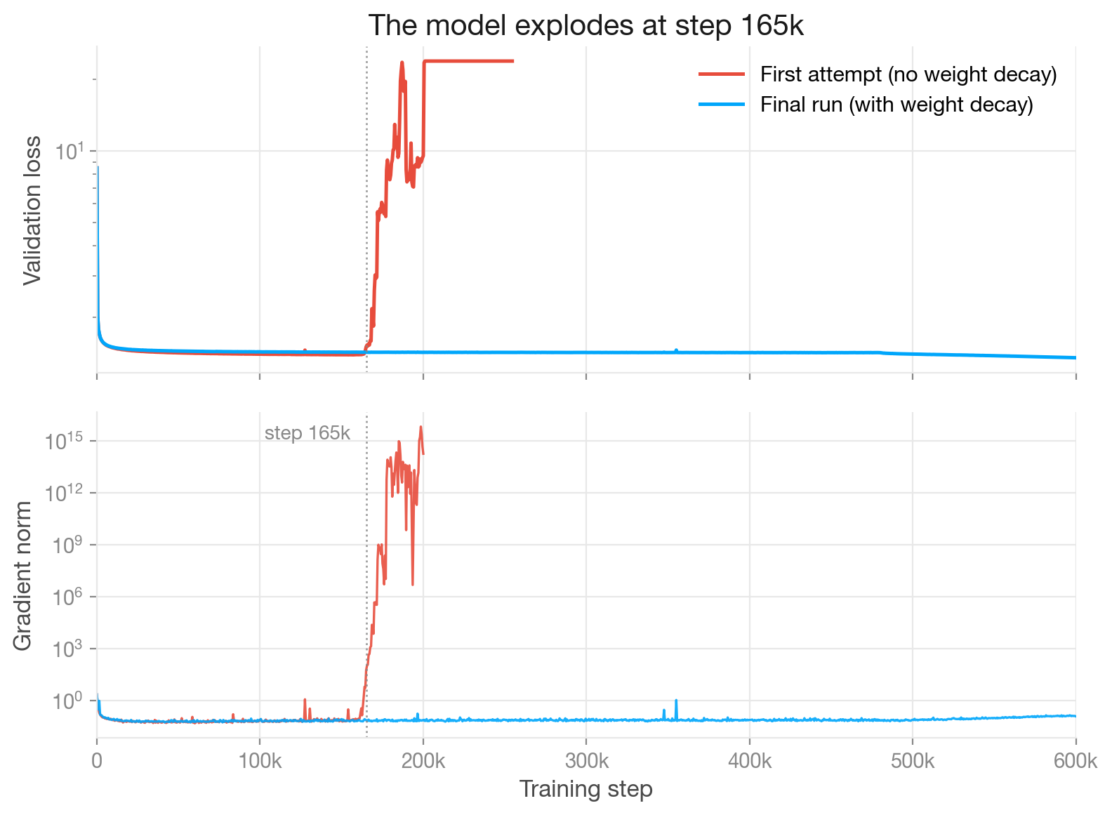
I first tried to rescue the run. Restarting from a healthy checkpoint with lower learning rates looked promising for a few thousand steps, but every variant either diverged again or showed the same upward bend in the loss. Whatever this was, lowering the learning rate only delayed it.
Digging through the checkpoints revealed something surprising: the failure was localized. In plain terms, one tiny part of the network started growing without limit and dragged everything else down with it. Specifically, a single channel in the LayerNorm before the attention of block 1 grew from 0.16 to 6.3 between steps 150k and 200k while its paired bias swung to -6.0, and the Muon updates to that block's attention projections concentrated on that same channel. One normalization channel and a handful of weight columns had entered a feedback loop, and they took the rest of the model down with them.
The recipe had inherited one more choice from modded-nanogpt that I never questioned: no weight decay. Nothing in the training was pushing back against a weight that only wants to grow. The fix was a small amount of weight decay (0.005 for AdamW, 0.01 for Muon, values inspired by the NanoGPT speedrun community): a gentle force that shrinks every weight toward zero on each step, so nothing can grow unchecked. Then restart from scratch.
So, can autocomplete play chess blindfolded?
In short, usually. From our original goal of 100% VPM, our model is able to achieve 99.93%, with a 99.99% top-1 valid move accuracy. Game end accuracy was worse, out of our stated goal of 100% GPA our model achieves 99.49%, with a total correct game end probability mass of 99.19%
These numbers are from evaluating the model in a large, balanced, held-out dataset. The dataset consists of 768,000 games it never saw during training: 768 buckets, 16 white ratings (1000-2500) x 16 black ratings (1000-2500) x 3 time controls (bullet, blitz, rapid), 1,000 games per bucket, drawn from 2022-2023. Classical is left out: there are not enough classical games in that window to fill all 768 buckets.
| Held-out metric (with metadata) | Bullet | Blitz | Rapid | Total |
|---|---|---|---|---|
| Cross-entropy over legal moves (nats) | 1.446 | 1.321 | 1.332 | 1.366 |
| Perplexity over legal moves | 4.25 | 3.75 | 3.79 | 3.92 |
| Valid move probability mass | 99.93% | 99.94% | 99.92% | 99.93% |
| Top-1 move = human's | 55.12% | 58.07% | 57.83% | 57.01% |
| Game-end prediction accuracy | 99.78% | 99.46% | 99.29% | 99.49% |
per_cell_metrics.csv.The two deep dives below explore where the remaining 0.07% VPM and 0.51% GPA are.
Deep diveWhere the model plays an illegal move
The top move is legal 99.99% of the time, yet the distribution still leaks 0.07% of its probability onto illegal ones, the gap under a 99.93% VPM.
92.6% of this 0.07% is the model choosing illegal moves. The remaining 7.4% is the model assigning probability to a game end token before the game has ended.
The type of illegal move with the most probability mass is leaving the king in check, followed by the move not being possible due to the path being blocked, and then the model attempting to move a piece that is not there.
The spurious game ends spread their probability mass fairly evenly across the ending types, with stalemate and the fifty-move rule the least likely.
A greedy player who always takes the model's top move meets a different slice: the 4,830 positions, out of 45.7M, where that top move is illegal. False game ends take 42.5% of this slice against 7.4% of the mass above. When the model calls a live game over it commits a large share of its probability, so the error weighs more under the top move than in the mass. The 1,534 spurious game ends here are the same false alarms the game end deep dive counts (Table 9).
Deep diveWhere the game end predictions fail
The 99.49% GPA pools easy endings with hard ones. The model nails the sharp, on-the-board endings and stumbles on the two that are rare or inconsistently drawn in the training data:
The misses split in two. A false alarm (calling a live game over) is the one to avoid, and it stays rare: across the 91,457,538 move predictions in the two scorings, with and without metadata, the model raised one 3,077 times, about 0.003%. Of those, 1,534 come from the with-metadata run below. The opposite error, missing a real ending and playing on, is what the 99.49% measures, and nearly all those misses land on threefold repetition and the fifty move rule.
Split across the 280,472 real terminal positions and the 45.7M ongoing ones, with metadata:
| Failure mode | Count | Rate |
|---|---|---|
| Real ending missed, played a move instead | 1,134 | 0.404% |
| Real ending not even in the model's top 5 | 203 | 0.072% |
| Right that it ended, wrong reason | 17 | 0.006% |
| False alarm (declared a live game over) | 1,534 | 0.003% |
The value of Elo and time control information
The metadata tokens were meant to let the model adapt to the players in front of it. Do they change how it plays? This is tested by scoring the model twice on the same games: once with all three metadata tokens present, once with every one replaced by . The gain is smallest when both players sit near the 1664 median, where the model already guesses the typical continuation, and largest when the players are far from average:
| White rating ↓ Black rating → | 1000–1300 | 1400–1700 | 1800–2100 | 2200–2500 |
|---|---|---|---|---|
| 1000–1300 | +0.81 | +0.86 | +1.32 | +2.03 |
| 1400–1700 | +0.78 | +0.39 | +0.62 | +1.29 |
| 1800–2100 | +1.12 | +0.53 | +0.43 | +0.85 |
| 2200–2500 | +1.76 | +1.19 | +0.85 | +0.99 |
The pattern shows the model acts on the rating tokens rather than ignoring them. Between two average players there is little to add: the no-metadata guess is already the common move. Tell it instead that a 1000 rated player is facing a 2400, and it shifts toward moves it would otherwise never reach, a pairing nothing in its no-metadata prior accounts for.
The coarse 4×4 heatmap (Figure 18) bins a finer 16×16 grid. The full version is in the appendix: the metadata gain (Figure 23), raw move match (Figure 24), and loss (Figure 25), cell by cell.
Playing strength
Deep diveHow playing strength is measured
The model plays Stockfish 18 at a range of Elo levels, and each game is scored for the model as a win, draw, or loss (1, ½, or 0). Games that finish on the board are scored by their result; a game that hits a cap of 200 half moves without ending is adjudicated by a full-strength Stockfish (Elo limiter off, single-threaded, search depth 18), scored as a win or loss once its evaluation passes 200 centipawns and a draw otherwise. The win, draw, and loss counts over all the games give the relative rating.
Each game is seeded with an opening rather than started from the empty board. Without that, a greedy model against fixed Stockfish settings would replay nearly the same game every time. The openings are the 32 most common lines (those most often reached in the training corpus, each taken at a fixed depth of four moves) and the 32 rarest, each followed as deep as needed to reach a line the model almost never saw. We keep only equal openings, meaning Stockfish gives neither side more than a 25-centipawn advantage in the position after the opening. That keeps a game turning on how the two sides play rather than on a lopsided position handed to one of them before its first choice. No opening is a continuation of another, so the 64 openings cover genuinely distinct lines; each is played twice in every configuration, once with the model as white and once as black, and 64 openings × 2 colors is where the 128 games per cell reported below come from. Both groups are listed in full below.
| ECO | Opening | Games | Eval | Moves |
|---|---|---|---|---|
| C57 | Italian Game: Two Knights Defense, Knight Attack, Normal Variation | 11,968,381 | +0.24 | 1. e4 e5 2. ♘︎f3 ♞︎c6 3. ♗︎c4 ♞︎f6 4. ♘︎g5 d5 |
| C54 | Italian Game: Classical Variation | 8,320,274 | +0.24 | 1. e4 e5 2. ♘︎f3 ♞︎c6 3. ♗︎c4 ♝︎c5 4. c3 ♞︎f6 |
| C50 | Italian Game: Giuoco Pianissimo, Normal | 7,706,006 | +0.22 | 1. e4 e5 2. ♘︎f3 ♞︎c6 3. ♗︎c4 ♞︎f6 4. d3 ♝︎c5 |
| C45 | Scotch Game: Schmidt Variation | 4,627,923 | +0.14 | 1. e4 e5 2. ♘︎f3 ♞︎c6 3. d4 exd4 4. ♘︎xd4 ♞︎f6 |
| C50 | Four Knights Game: Italian Variation | 3,689,342 | +0.18 | 1. e4 e5 2. ♘︎f3 ♞︎c6 3. ♗︎c4 ♝︎c5 4. ♘︎c3 ♞︎f6 |
| C47 | Four Knights Game: Scotch Variation Accepted | 3,532,392 | +0.07 | 1. e4 e5 2. ♘︎f3 ♞︎c6 3. ♘︎c3 ♞︎f6 4. d4 exd4 |
| C51 | Italian Game: Evans Gambit Accepted | 2,993,907 | -0.21 | 1. e4 e5 2. ♘︎f3 ♞︎c6 3. ♗︎c4 ♝︎c5 4. b4 ♝︎xb4 |
| D53 | Queen's Gambit Declined | 2,542,137 | +0.13 | 1. d4 d5 2. c4 e6 3. ♘︎c3 ♞︎f6 4. ♗︎g5 ♝︎e7 |
| C44 | Scotch Game: Haxo Gambit | 2,382,962 | +0.07 | 1. e4 e5 2. ♘︎f3 ♞︎c6 3. d4 exd4 4. ♗︎c4 ♝︎c5 |
| B13 | Caro-Kann Defense: Exchange Variation | 2,314,558 | +0.24 | 1. e4 c6 2. d4 d5 3. exd5 cxd5 4. ♘︎f3 ♞︎c6 |
| C44 | Scotch Game: Scotch Gambit, Dubois Réti Defense | 2,279,040 | +0.05 | 1. e4 e5 2. ♘︎f3 ♞︎c6 3. ♗︎c4 ♞︎f6 4. d4 exd4 |
| C22 | Center Game: Berger Variation | 1,621,763 | -0.18 | 1. e4 e5 2. d4 exd4 3. ♕︎xd4 ♞︎c6 4. ♕︎e3 ♞︎f6 |
| B22 | Sicilian Defense: Alapin Variation, Smith-Morra Declined | 1,022,691 | +0.20 | 1. e4 c5 2. c3 ♞︎f6 3. e5 ♞︎d5 4. d4 cxd4 |
| B24 | Sicilian Defense: Closed | 798,689 | -0.02 | 1. e4 c5 2. ♘︎c3 ♞︎c6 3. g3 g6 4. ♗︎g2 ♝︎g7 |
| C44 | Scotch Game: Scotch Gambit, London Defense | 767,016 | +0.03 | 1. e4 e5 2. ♘︎f3 ♞︎c6 3. d4 exd4 4. ♗︎c4 ♝︎b4+ |
| C49 | Four Knights Game: Spanish Variation, Double Spanish | 725,017 | +0.17 | 1. e4 e5 2. ♘︎f3 ♞︎c6 3. ♘︎c3 ♞︎f6 4. ♗︎b5 ♝︎b4 |
| A48 | London System | 481,292 | +0.18 | 1. d4 ♞︎f6 2. ♘︎f3 g6 3. ♗︎f4 ♝︎g7 4. e3 d6 |
| E46 | Nimzo-Indian Defense: Normal Variation | 473,960 | +0.19 | 1. d4 ♞︎f6 2. c4 e6 3. ♘︎c3 ♝︎b4 4. e3 O-O |
| C48 | Four Knights Game: Spanish Variation, Rubinstein Variation | 319,315 | +0.10 | 1. e4 e5 2. ♘︎f3 ♞︎c6 3. ♘︎c3 ♞︎f6 4. ♗︎b5 ♞︎d4 |
| D38 | Queen's Gambit Declined: Ragozin Defense | 318,441 | +0.24 | 1. d4 ♞︎f6 2. c4 e6 3. ♘︎f3 d5 4. ♘︎c3 ♝︎b4 |
| E34 | Nimzo-Indian Defense: Classical Variation, Noa Variation | 296,038 | +0.16 | 1. d4 ♞︎f6 2. c4 e6 3. ♘︎c3 ♝︎b4 4. ♕︎c2 d5 |
| B10 | Caro-Kann Defense: Accelerated Panov Attack, Modern Variation | 261,433 | +0.12 | 1. e4 c6 2. c4 d5 3. exd5 cxd5 4. cxd5 ♞︎f6 |
| C36 | King's Gambit Accepted: Abbazia Defense | 216,096 | -0.22 | 1. e4 e5 2. f4 exf4 3. ♘︎f3 d5 4. exd5 ♞︎f6 |
| C07 | French Defense: Tarrasch Variation, Chistyakov Defense | 211,808 | +0.19 | 1. e4 e6 2. d4 d5 3. ♘︎d2 c5 4. exd5 ♛︎xd5 |
| C44 | Scotch Game: Scotch Gambit, Göring Gambit Declined | 197,073 | +0.03 | 1. e4 e5 2. ♘︎f3 ♞︎c6 3. d4 exd4 4. c3 d5 |
| A48 | Indian Defense: Colle System, King's Indian Variation | 191,400 | +0.22 | 1. d4 ♞︎f6 2. ♘︎f3 g6 3. e3 ♝︎g7 4. ♗︎d3 d6 |
| D04 | Queen's Pawn Game: Colle System, Grünfeld Formation | 138,514 | -0.15 | 1. d4 d5 2. ♘︎f3 ♞︎f6 3. e3 g6 4. ♗︎d3 ♝︎g7 |
| A25 | English Opening: King's English Variation, Taimanov Variation | 93,747 | +0.22 | 1. c4 e5 2. ♘︎c3 ♞︎c6 3. g3 g6 4. ♗︎g2 ♝︎g7 |
| A23 | English Opening: King's English Variation, Two Knights Variation, Keres Variation | 80,311 | +0.16 | 1. c4 e5 2. ♘︎c3 ♞︎f6 3. g3 ♝︎c5 4. ♗︎g2 c6 |
| D00 | Blackmar-Diemer Gambit Declined: Lamb Defense | 77,192 | -0.17 | 1. d4 d5 2. e4 dxe4 3. ♘︎c3 ♞︎f6 4. f3 ♞︎c6 |
| A36 | English Opening: Symmetrical Variation, Ultra-Symmetrical Variation | 72,407 | +0.25 | 1. c4 c5 2. g3 g6 3. ♗︎g2 ♝︎g7 4. ♘︎c3 ♞︎c6 |
| A48 | Queen's Pawn Game: Barry Attack | 71,768 | +0.00 | 1. d4 ♞︎f6 2. ♘︎f3 g6 3. ♘︎c3 d5 4. ♗︎f4 ♝︎g7 |
| ECO | Opening | Games | Eval | Moves |
|---|---|---|---|---|
| A33 | English Opening: Symmetrical Variation, Anti-Benoni Variation, Geller Variation | 0 | +0.08 | 1. c4 e6 2. ♘︎f3 ♞︎f6 3. ♘︎c3 c5 4. d4 ♞︎c6 5. g3 cxd4 6. ♘︎xd4 ♛︎b6 |
| B74 | Sicilian Defense: Dragon Variation, Classical Variation, Stockholm Attack | 0 | -0.16 | 1. e4 c5 2. ♘︎c3 d6 3. f4 ♞︎c6 4. ♘︎f3 g6 5. d4 cxd4 6. ♘︎xd4 ♝︎g7 7. ♗︎e3 ♞︎f6 8. ♗︎e2 O-O 9. ♘︎b3 ♝︎e6 10. O-O ♞︎a5 11. f5 ♝︎c4 12. ♘︎xa5 ♝︎xe2 13. ♕︎xe2 ♛︎xa5 14. g4 |
| D34 | Tarrasch Defense: Classical Variation, Bogoljubow Variation | 0 | +0.24 | 1. d4 ♞︎f6 2. c4 e6 3. ♘︎c3 c5 4. ♘︎f3 d5 5. cxd5 exd5 6. g3 ♞︎c6 7. ♗︎g2 ♝︎e7 8. O-O O-O 9. ♗︎g5 ♝︎e6 10. ♖︎c1 c4 |
| D49 | Semi-Slav Defense: Meran Variation, Rellstab Attack | 0 | +0.01 | 1. d4 d5 2. c4 c6 3. ♘︎c3 ♞︎f6 4. ♘︎f3 e6 5. e3 ♞︎bd7 6. ♗︎d3 dxc4 7. ♗︎xc4 b5 8. ♗︎d3 a6 9. e4 c5 10. e5 cxd4 11. ♘︎xb5 ♞︎xe5 12. ♘︎xe5 axb5 13. O-O ♛︎d5 14. ♕︎e2 ♝︎a6 15. ♗︎g5 |
| D64 | Queen's Gambit Declined: Orthodox Defense, Rubinstein Attack | 0 | +0.22 | 1. d4 ♞︎f6 2. c4 e6 3. ♘︎c3 d5 4. ♘︎f3 ♝︎e7 5. ♗︎g5 O-O 6. e3 ♞︎bd7 7. ♖︎c1 c6 8. a3 a6 9. ♕︎c2 |
| D68 | Queen's Gambit Declined: Orthodox Defense, Classical Variation | 0 | +0.09 | 1. d4 d5 2. c4 e6 3. ♘︎f3 ♞︎f6 4. ♘︎c3 ♝︎e7 5. ♗︎g5 O-O 6. e3 ♞︎bd7 7. ♖︎c1 c6 8. ♗︎d3 dxc4 9. ♗︎xc4 ♞︎d5 10. ♗︎xe7 ♛︎xe7 11. O-O ♞︎xc3 12. ♖︎xc3 e5 13. ♕︎b1 |
| E08 | Catalan Opening: Closed, Zagoryansky Variation | 0 | +0.18 | 1. d4 e6 2. c4 ♞︎f6 3. ♘︎f3 d5 4. g3 ♝︎e7 5. ♗︎g2 O-O 6. O-O ♞︎bd7 7. ♕︎c2 c6 8. ♖︎d1 b6 9. a4 |
| A30 | English Opening: Symmetrical, Hedgehog, Flexible Formation | 1 | +0.22 | 1. c4 e6 2. ♘︎f3 c5 3. ♘︎c3 ♞︎f6 4. g3 b6 5. ♗︎g2 ♝︎b7 6. O-O ♝︎e7 7. d4 cxd4 8. ♕︎xd4 d6 9. ♖︎d1 a6 10. b3 ♞︎bd7 |
| B51 | Sicilian Defense: Moscow Variation, Dorfman Gambit | 1 | -0.06 | 1. e4 c5 2. ♘︎f3 d6 3. ♗︎b5+ ♞︎c6 4. O-O ♝︎d7 5. ♕︎e2 g6 6. e5 |
| D12 | Slav Defense: Quiet Variation, Landau Variation | 1 | -0.25 | 1. d4 d5 2. c4 c6 3. ♘︎f3 ♞︎f6 4. e3 ♝︎f5 5. cxd5 cxd5 6. ♕︎b3 ♛︎c8 7. ♗︎d2 e6 8. ♘︎a3 |
| D26 | Queen's Gambit Accepted: Classical, Furman Variation | 1 | -0.05 | 1. d4 d5 2. c4 dxc4 3. ♘︎f3 ♞︎f6 4. e3 e6 5. ♗︎xc4 c5 6. ♕︎e2 a6 7. dxc5 ♝︎xc5 8. O-O ♞︎c6 9. e4 b5 10. e5 |
| D28 | Queen's Gambit Accepted: Classical, Flohr Variation | 1 | +0.00 | 1. d4 d5 2. c4 dxc4 3. ♘︎f3 ♞︎f6 4. e3 e6 5. ♗︎xc4 c5 6. O-O a6 7. ♕︎e2 b5 8. ♗︎b3 ♞︎c6 9. ♖︎d1 c4 10. ♗︎c2 ♞︎b4 11. ♘︎c3 ♞︎xc2 12. ♕︎xc2 ♝︎b7 13. d5 ♛︎c7 |
| D49 | Semi-Slav Defense: Meran Variation, Stahlberg Variation | 1 | +0.22 | 1. d4 d5 2. c4 c6 3. ♘︎c3 ♞︎f6 4. e3 e6 5. ♘︎f3 ♞︎bd7 6. ♗︎d3 dxc4 7. ♗︎xc4 b5 8. ♗︎d3 a6 9. e4 c5 10. e5 cxd4 11. ♘︎xb5 ♞︎xe5 12. ♘︎xe5 axb5 13. ♕︎f3 |
| C41 | Philidor Defense: Lopez Countergambit, Jaenisch Variation | 2 | +0.00 | 1. e4 e5 2. ♘︎f3 d6 3. d4 f5 4. ♗︎c4 exd4 5. ♘︎g5 ♞︎h6 6. ♘︎xh7 |
| C42 | Petrov's Defense: Classical Attack, Maróczy Variation | 2 | -0.12 | 1. e4 e5 2. ♘︎f3 ♞︎f6 3. ♘︎xe5 d6 4. ♘︎f3 ♞︎xe4 5. d4 d5 6. ♗︎d3 ♝︎e7 7. O-O ♞︎c6 8. ♖︎e1 ♝︎g4 9. c3 f5 10. c4 ♝︎h4 |
| B06 | Pterodactyl Defense: Fianchetto, King Pterodactyl | 4 | +0.20 | 1. e4 g6 2. d4 ♝︎g7 3. g3 c5 4. ♘︎f3 ♛︎a5+ |
| A45 | Trompowsky Attack: Edge Variation, Hergert Gambit | 5 | +0.24 | 1. d4 ♞︎f6 2. ♗︎g5 ♞︎e4 3. ♗︎h4 c6 4. ♘︎d2 ♛︎a5 5. c3 ♞︎xd2 6. ♕︎xd2 d5 7. e4 |
| C33 | King's Gambit Accepted: Bishop's Gambit, Fraser Variation | 5 | -0.24 | 1. e4 e5 2. f4 exf4 3. ♗︎c4 ♛︎h4+ 4. ♔︎f1 g5 5. ♘︎c3 ♝︎g7 6. g3 fxg3 7. ♕︎f3 |
| D35 | Queen's Gambit Declined: Exchange Variation, Chameleon Variation | 5 | -0.22 | 1. d4 ♞︎f6 2. c4 e6 3. ♘︎c3 d5 4. cxd5 exd5 5. ♗︎g5 ♝︎e7 6. e3 O-O 7. ♗︎d3 ♞︎bd7 8. ♕︎c2 ♜︎e8 9. ♘︎ge2 ♞︎f8 10. O-O-O |
| D98 | Grünfeld Defense: Russian Variation, Keres Variation | 6 | +0.20 | 1. d4 ♞︎f6 2. c4 g6 3. ♘︎c3 d5 4. ♘︎f3 ♝︎g7 5. ♕︎b3 dxc4 6. ♕︎xc4 O-O 7. e4 ♝︎g4 8. ♗︎e3 ♞︎fd7 9. ♗︎e2 ♞︎b6 10. ♕︎d3 ♞︎c6 11. O-O-O |
| E08 | Catalan Opening: Closed | 6 | +0.25 | 1. d4 ♞︎f6 2. c4 e6 3. g3 d5 4. ♗︎g2 ♝︎e7 5. ♘︎f3 O-O 6. O-O ♞︎bd7 7. ♕︎c2 c6 8. ♗︎f4 b6 9. ♘︎bd2 ♝︎b7 10. e4 |
| E29 | Nimzo-Indian Defense: Sämisch Variation, Capablanca Variation | 6 | -0.05 | 1. d4 ♞︎f6 2. c4 e6 3. ♘︎c3 ♝︎b4 4. e3 c5 5. ♗︎d3 ♞︎c6 6. a3 ♝︎xc3+ 7. bxc3 O-O 8. ♘︎e2 b6 9. e4 ♞︎e8 |
| C88 | Ruy Lopez: Closed, Alekhine Gambit | 7 | +0.00 | 1. e4 e5 2. ♘︎f3 ♞︎c6 3. ♗︎b5 a6 4. ♗︎a4 ♞︎f6 5. O-O ♝︎e7 6. ♖︎e1 b5 7. ♗︎b3 d6 8. c3 ♞︎a5 9. ♗︎c2 c5 10. d4 ♛︎c7 11. ♘︎bd2 O-O 12. ♘︎f1 ♝︎g4 13. ♘︎e3 ♝︎xf3 14. ♕︎xf3 |
| D67 | Queen's Gambit Declined: Orthodox Defense, Janowski Variation | 7 | +0.25 | 1. d4 d5 2. ♘︎f3 ♞︎f6 3. c4 e6 4. ♘︎c3 ♝︎e7 5. ♗︎g5 O-O 6. e3 ♞︎bd7 7. ♖︎c1 c6 8. ♗︎d3 dxc4 9. ♗︎xc4 ♞︎d5 10. h4 |
| E14 | Queen's Indian Defense: Averbakh Variation | 7 | +0.02 | 1. d4 ♞︎f6 2. c4 e6 3. ♘︎f3 b6 4. e3 ♝︎b7 5. ♗︎d3 c5 6. O-O ♝︎e7 7. b3 O-O 8. ♗︎b2 cxd4 9. ♘︎xd4 |
| D40 | Queen's Gambit Declined: Semi-Tarrasch Defense, Levenfish Variation | 8 | -0.03 | 1. d4 d5 2. c4 e6 3. ♘︎c3 ♞︎f6 4. ♘︎f3 c5 5. e3 ♞︎c6 6. ♗︎d3 ♝︎d6 7. O-O O-O 8. ♕︎e2 ♛︎e7 9. dxc5 ♝︎xc5 10. e4 |
| D49 | Semi-Slav Defense: Meran Variation, Sozin Variation | 8 | +0.00 | 1. d4 d5 2. ♘︎f3 ♞︎f6 3. c4 c6 4. ♘︎c3 e6 5. e3 ♞︎bd7 6. ♗︎d3 dxc4 7. ♗︎xc4 b5 8. ♗︎d3 a6 9. e4 c5 10. e5 cxd4 11. ♘︎xb5 ♞︎xe5 12. ♘︎xe5 axb5 13. O-O |
| D19 | Slav Defense: Czech Variation, Dutch Variation, Sämisch Variation | 9 | +0.20 | 1. d4 d5 2. c4 c6 3. ♘︎f3 ♞︎f6 4. ♘︎c3 dxc4 5. a4 ♝︎f5 6. e3 e6 7. ♗︎xc4 ♝︎b4 8. O-O O-O 9. ♕︎e2 ♞︎e4 10. g4 |
| E63 | King's Indian Defense: Fianchetto Variation, Panno Variation, Korchnoi Line | 9 | +0.12 | 1. d4 ♞︎f6 2. c4 g6 3. ♘︎f3 ♝︎g7 4. g3 O-O 5. ♗︎g2 d6 6. O-O ♞︎c6 7. ♘︎c3 a6 8. h3 ♜︎b8 9. ♗︎e3 b5 10. ♘︎d2 |
| E42 | Nimzo-Indian Defense: Rubinstein System, Rubinstein Variation, Sherbakov Attack | 10 | -0.05 | 1. d4 ♞︎f6 2. c4 e6 3. ♘︎c3 ♝︎b4 4. e3 c5 5. ♘︎e2 cxd4 6. exd4 O-O 7. c5 |
| A40 | English Defense: Hartlaub Gambit Declined | 12 | +0.17 | 1. c4 e6 2. d4 b6 3. ♘︎c3 ♝︎b7 4. e4 f5 5. d5 |
| C15 | French Defense: Winawer Variation, Fingerslip Variation, Schwarz's Line | 12 | -0.19 | 1. e4 e6 2. d4 d5 3. ♘︎c3 ♝︎b4 4. ♗︎d2 ♞︎e7 5. ♘︎b1 |
The rating in each cell is a performance rating: the Elo you would need to score that result against that one fixed opponent, read off the standard (FIDE) rating-difference table, the same method Allie uses. Because it depends only on the win/draw/loss totals, not the order the games were played, it is order-independent and reproducible. The ± is one standard error of the score, mapped onto the Elo scale.
The five opponents in the final 46,080-game evaluation are not one Stockfish run at different depths. Each level is a distinct configuration, a search-depth cap plus a time budget per move, and the Elo shown is the nominal rating attached to that configuration:
| Level | Pinned Elo | Depth cap | Time / move | Threads |
|---|---|---|---|---|
| 0 | 1347 | 5 | 126 ms | 1 |
| 3 | 1729 | 5 | 168 ms | 1 |
| 7 | 2518 | 5 | 253 ms | 1 |
| 11 | 2851 | 8 | 337 ms | 1 |
| 16 | 3099 | 12 | 422 ms | 1 |
The model itself plays greedily during evaluation (it always takes its single most likely legal move, no sampling). The depth caps and per-move times come from Lichess's fishnet client, and the Elo labels are Stockfish's own published skill-level ratings, interpolated to each level. Those Elo figures are labels for the configurations rather than a calibrated human scale, so a rating read off this ladder should be read as "relative to this ladder," not as a Lichess or FIDE number.
To measure strength the model played 46,080 games against Stockfish at five capped levels across openings and all four time controls, with long games adjudicated by a full-strength Stockfish. The model plays greedily: its single most likely legal move, no search. It is conditioned on a time control too, so each figure shows a single time control; this one is classical. Conditioned on a 2500 rating, the top of our grid, it scores:
Each of those scores converts to a performance rating: the Elo you would need to score that much against that one opponent. For the 2500-conditioned model in classical:
The conditioned rating has only a minor effect on the performance rating of the model, and the effect disappears against stronger opponents. The factor that most affects the model's playing strength is its opponent. The stronger the opponent, the better the model plays. Greedy play also sets a floor on how weak the model can be. Its output is a poll of every 1000 rated player it has seen, and they blunder in different ways: the mistakes scatter across many moves while the reasonable move collects the most mass, so always playing the top move amounts to taking the crowd's vote. Even conditioned as a 1000, the model lands around 1600 against the weakest ladder level.
By default each line is one conditioned rating, drawn across the Stockfish ladder. The X axis control flips that: one line per Stockfish level, drawn across the conditioned ratings, with No metadata as a trailing column, so the chart reads two ways, across the ladder or across conditioning. Hover a column to read off every visible line with its wins, draws, and losses. Each point pools 128 games (the no-metadata line 1,152); the All time-control view pools all four controls into 512 (no metadata 4,608). Filtering to one opening family or one color halves the count, both together quarter it, and the whiskers widen to match. The dashed reference marks an even 50% score, or in the rating view the opponent's own Elo (shown only in the default Stockfish-x orientation). The same numbers, exact and cell by cell, are in the strength table (Figure 22).
Deep divePlaying strength, in detail
The table holds every conditioned rating against every Stockfish level, in classical games, 128 games per cell, with metadata; the bars above are its 2500 row. Its controls switch the metric (score, W/D/L, or performance rating), the time control, the opening family, and the colour the model played, and add a no-metadata row.
Conditioning helps, but only within a band: in the weak and middle columns the cells get greener from the 1000 row up to 2500, and in the two strongest columns that gain is gone, the 2500-conditioned model no greener than the 1000-conditioned one, both red.
Turned into performance ratings (the Elo needed to score each result against that one opponent), the model traces a slope rather than settling on a number. The 2500-conditioned model rates about 1817 against the weakest Stockfish and about 2716 against the strongest, a ~900-point spread for one fixed model. Conditioning also matters most against weak opponents: on the rating metric the lines fan out about 240 points against the weakest engine and collapse to about 70 against the strongest. Switch Figure 21 to the performance-rating metric to see both. These are ratings on this Stockfish ladder, not a Lichess or FIDE scale.
How all 46,080 games ended:
| Game ending | Count | Share |
|---|---|---|
| Checkmate | 36,686 | 79.6% |
| Threefold repetition | 6,672 | 14.5% |
| Stalemate | 696 | 1.5% |
| Insufficient material | 367 | 0.8% |
| Fifty move rule | 10 | 0.0% |
| Adjudicated at the 200-move cap | 1,649 | 3.6% |
| Total games | 46,080 |
Over three quarters end in checkmate on the board; threefold repetition is next at 14.5%, and only 3.6% needed adjudication at the 200-move cap.
An important caveat: these are results against specific configurations of Stockfish, not against humans. An engine chooses moves nothing like a person does, so a score against it says how the model performs in that match-up, not how it would do against a human of any given rating.
How does it compare to the state of the art?
There is a line of research focused on chess models that are able to play chess like a human would. Given that our model is trained on an enormous amount of human games, we should expect it to do quite well on this task. The standard benchmark is the test set released with Allie (884,049 Lichess blitz positions) scored by how often a system's top move equals the move the human actually played.
| System | Move match |
|---|---|
| chess-autocomplete-v1 (700M, 61.4B tokens) | 57.2% |
| Maia-3 (79M, 2026) † | 57.1% |
| chess-autocomplete-v1 (350M) | 57.0% |
| Maia-3 (23M, 2026) † | 56.6% |
| chess-autocomplete-v1 (91M) | 56.0% |
| Allie (adaptive search, 2024) † ⚙ | 55.9% |
| Allie (policy, 2024) † | 55.7% |
| Maia-3 (5M, 2026) † | 55.4% |
| GPT-3.5 (2023) † | 53.7% |
| Maia-2 (2024) † | 52.0% |
| Maia⋆ (rating-matched, 2020) † | 51.6% |
The 700M takes the top spot on half the data: it is the T=300k anneal branch, 61.4B tokens against the 122.9B the other two each saw. The 350M lands third, a tenth of a point under Maia-3's 79M variant. The 91M sits fifth, with four rows above it, two of them our own larger models and two the largest Maia-3 variants (23M and 79M, released in May 2026); it still lands ahead of Allie, GPT-3.5, Maia-2, and the rating-matched original Maia.
That leaderboard is blitz. Maia-2 measures the same skill on rapid, its Maia-1 test set, where the moving player's rating splits the games into Skilled, Advanced, and Master. Both our models lead Maia-2 in every group:
| Model | Skilled | Advanced | Master | Avg |
|---|---|---|---|---|
| Maia-2 | 51.72 | 54.15 | 53.87 | 53.25 |
| Ours (91M) | 56.69 | 59.39 | 60.90 | 58.99 |
| Ours (350M) | 57.40 | 60.34 | 62.17 | 59.97 |
The remaining reproductions, Maia-2's cross-skill grid, Allie's move-legality and move-type tables, and a breakdown of where the 56% comes from, are in the appendix.
Blindfolded, and near the top
The question was whether a model that reads nothing but a stream of moves, with no board in front of it and no rules to consult, could play chess blindfolded. It can.
On our held-out set of games it never saw, 99.93% of its probability lands on legal moves, and it correctly determines when a game has ended 99.49% of the time. It hasn't learned the rules perfectly, but almost.
On the standard human move benchmark it matches 56% of the moves real players chose, behind only the two largest Maia-3 networks and ahead of every Maia, Maia-2, Allie, and GPT-3.5 entry. That is 91M parameters, with none of the machinery the others lean on. These benchmarks each cover one thin slice of chess. The Allie set is blitz, its openings and time-scramble moves thrown out; the Maia-2 set is rapid, split into rating bands. The models behind them are narrow to begin with: Allie and Maia-3 trained on blitz alone, Maia-2 on rapid. Ours saw all of it, four time controls from bullet to classical and every rating, nothing held back, and it still scores near the top on their slice.
And all of this was achieved by simply:
predicting the next token
That board at the top? It's the full model
The board at the top of this page is the real thing: the full 91M parameter model running in your browser through ONNX Runtime with WebGPU. At each move the model produces a probability distribution over moves; illegal moves are masked out, and by default it plays its most likely legal move (you can switch on temperature and top-k sampling in the settings to make it less predictable). The interface handles the FIDE draw rules. By default the model is conditioned as a 2500 rated rapid player, the top rating bucket, and the same 2500 rating the strength numbers above used (those were in classical, this board is rapid). Good luck.
Get the model, dataset, and code
Everything in this post is open:
- The model, in PyTorch, safetensors and ONNX formats: Alfredvc/chess-autocomplete-v1-91m
- The larger models: Alfredvc/chess-autocomplete-v1-350m and Alfredvc/chess-autocomplete-v1-700m-300k
- The processed dataset: Alfredvc/chess-autocomplete-lichess
- The evaluation datasets: Alfredvc/chess-autocomplete-eval-datasets
- The training checkpoints, with optimizer state and training curves: Alfredvc/chess-autocomplete-v1-checkpoints
- The full training and evaluation code: Alfredvc/chess-autocomplete
References
- Lichess open database
- Chessformer: A Unified Architecture for Chess Modeling (Maia-3)
- Maia-2: A Unified Model for Human-AI Alignment in Chess
- Human-aligned Chess with a Bit of Search (Allie)
- Aligning Superhuman AI with Human Behavior: Chess as a Model System (Maia)
- Amortized Planning with Large-Scale Transformers: A Case Study on Chess (Grandmaster-Level Chess Without Search)
- Muon optimizer
- modded-nanogpt
- FlashAttention
- Scaling Laws and Compute-Optimal Training Beyond Fixed Training Durations
- FIDE Rating Regulations (performance-rating conversion table, §8.1.1)
- Language Models are Unsupervised Multitask Learners (GPT-2)
Appendix
The full rating×rating grids
The coarse 4×4 heatmap in The value of Elo and time control information bins a finer 16×16 grid. Here is the full version, all with metadata, white rating down the rows and black rating across the columns: the metadata gain (Figure 23), brightest at the corners; raw move match (Figure 24), which rises with rating because stronger players are more predictable; and the loss (Figure 25), which falls the same way. On a narrow screen the grids scroll sideways.
| W ↓ / B → | 1000 | 1100 | 1200 | 1300 | 1400 | 1500 | 1600 | 1700 | 1800 | 1900 | 2000 | 2100 | 2200 | 2300 | 2400 | 2500 |
|---|---|---|---|---|---|---|---|---|---|---|---|---|---|---|---|---|
| 1000 | +1.07 | +0.90 | +0.93 | +1.19 | +1.15 | +1.18 | +1.23 | +1.24 | +1.45 | +1.56 | +1.79 | +2.09 | +2.16 | +2.18 | +2.31 | +2.42 |
| 1100 | +0.71 | +0.70 | +0.69 | +0.74 | +0.82 | +0.87 | +0.85 | +1.11 | +1.33 | +1.10 | +1.36 | +1.90 | +1.92 | +2.02 | +2.10 | +2.19 |
| 1200 | +0.94 | +0.78 | +0.67 | +0.73 | +0.75 | +0.64 | +0.75 | +0.76 | +0.88 | +1.04 | +1.12 | +1.52 | +1.86 | +1.94 | +2.12 | +2.28 |
| 1300 | +0.91 | +0.80 | +0.66 | +0.60 | +0.54 | +0.62 | +0.61 | +0.59 | +0.76 | +0.90 | +1.06 | +1.32 | +1.49 | +1.87 | +1.82 | +1.86 |
| 1400 | +1.01 | +0.77 | +0.69 | +0.64 | +0.56 | +0.49 | +0.37 | +0.50 | +0.51 | +0.71 | +0.84 | +1.16 | +1.37 | +1.59 | +1.77 | +1.87 |
| 1500 | +0.99 | +0.74 | +0.66 | +0.58 | +0.40 | +0.48 | +0.39 | +0.31 | +0.44 | +0.61 | +0.63 | +0.93 | +0.91 | +1.21 | +1.24 | +1.62 |
| 1600 | +1.02 | +0.82 | +0.74 | +0.55 | +0.43 | +0.29 | +0.28 | +0.24 | +0.31 | +0.43 | +0.72 | +0.80 | +0.76 | +1.11 | +1.33 | +1.38 |
| 1700 | +1.12 | +0.86 | +0.68 | +0.66 | +0.47 | +0.47 | +0.24 | +0.25 | +0.25 | +0.27 | +0.65 | +0.71 | +0.72 | +1.10 | +1.23 | +1.38 |
| 1800 | +1.22 | +0.93 | +0.87 | +0.81 | +0.52 | +0.44 | +0.29 | +0.22 | +0.27 | +0.29 | +0.56 | +0.65 | +0.83 | +0.89 | +0.99 | +1.17 |
| 1900 | +1.35 | +0.86 | +1.01 | +0.90 | +0.72 | +0.49 | +0.34 | +0.31 | +0.25 | +0.24 | +0.42 | +0.65 | +0.55 | +0.85 | +0.92 | +1.12 |
| 2000 | +1.49 | +1.27 | +1.12 | +0.89 | +0.82 | +0.62 | +0.48 | +0.43 | +0.36 | +0.31 | +0.48 | +0.47 | +0.51 | +0.71 | +0.89 | +1.17 |
| 2100 | +1.36 | +1.49 | +1.28 | +1.08 | +0.88 | +0.83 | +0.60 | +0.54 | +0.47 | +0.43 | +0.53 | +0.59 | +0.52 | +0.67 | +0.81 | +1.08 |
| 2200 | +1.73 | +1.61 | +1.42 | +1.46 | +1.15 | +0.85 | +0.79 | +0.69 | +0.59 | +0.62 | +0.69 | +0.46 | +0.56 | +0.78 | +0.87 | +1.11 |
| 2300 | +1.83 | +1.91 | +1.57 | +1.44 | +1.39 | +1.08 | +0.96 | +0.92 | +0.75 | +0.73 | +0.78 | +0.70 | +0.69 | +0.75 | +0.92 | +0.99 |
| 2400 | +2.09 | +1.74 | +1.73 | +1.61 | +1.49 | +1.29 | +1.28 | +1.15 | +1.02 | +0.87 | +0.82 | +0.88 | +0.91 | +0.91 | +1.15 | +1.19 |
| 2500 | +2.11 | +2.11 | +1.80 | +1.96 | +1.73 | +1.52 | +1.52 | +1.31 | +1.26 | +1.09 | +1.12 | +1.20 | +1.14 | +1.23 | +1.32 | +1.40 |
| W ↓ / B → | 1000 | 1100 | 1200 | 1300 | 1400 | 1500 | 1600 | 1700 | 1800 | 1900 | 2000 | 2100 | 2200 | 2300 | 2400 | 2500 |
|---|---|---|---|---|---|---|---|---|---|---|---|---|---|---|---|---|
| 1000 | 50.9 | 52.5 | 51.9 | 51.8 | 52.3 | 51.9 | 52.6 | 53.1 | 53.5 | 53.9 | 53.8 | 54.1 | 54.9 | 54.9 | 55.5 | 55.4 |
| 1100 | 52.6 | 53.5 | 54.1 | 53.1 | 53.3 | 53.1 | 53.9 | 54.4 | 54.6 | 54.5 | 55.4 | 55.7 | 56.0 | 56.1 | 56.2 | 56.4 |
| 1200 | 51.6 | 54.2 | 54.6 | 54.7 | 54.4 | 53.7 | 54.2 | 54.2 | 54.8 | 55.9 | 55.6 | 56.1 | 56.8 | 56.8 | 57.2 | 57.4 |
| 1300 | 51.7 | 53.3 | 54.9 | 55.7 | 55.6 | 54.6 | 55.0 | 54.7 | 55.4 | 55.8 | 56.3 | 56.8 | 57.1 | 57.3 | 57.5 | 57.3 |
| 1400 | 52.5 | 53.6 | 54.6 | 55.6 | 56.1 | 56.0 | 55.3 | 55.8 | 55.9 | 56.2 | 56.4 | 56.8 | 57.4 | 57.6 | 57.8 | 57.9 |
| 1500 | 52.0 | 53.5 | 53.8 | 54.9 | 56.0 | 56.4 | 56.3 | 55.8 | 56.1 | 56.8 | 56.6 | 57.1 | 57.5 | 57.8 | 57.5 | 57.8 |
| 1600 | 52.7 | 54.1 | 54.3 | 55.2 | 55.7 | 56.5 | 56.9 | 56.9 | 56.7 | 57.2 | 57.2 | 57.6 | 57.8 | 58.2 | 58.6 | 58.2 |
| 1700 | 53.2 | 54.4 | 54.4 | 55.5 | 55.6 | 56.1 | 57.1 | 57.1 | 57.5 | 57.2 | 57.7 | 58.1 | 58.3 | 58.8 | 58.8 | 59.1 |
| 1800 | 53.8 | 55.0 | 54.9 | 55.9 | 56.0 | 56.8 | 56.6 | 57.6 | 58.0 | 57.9 | 58.1 | 57.9 | 58.7 | 58.8 | 58.9 | 58.9 |
| 1900 | 54.3 | 55.1 | 55.8 | 56.3 | 56.5 | 56.8 | 56.9 | 57.5 | 58.0 | 58.3 | 58.4 | 58.4 | 58.8 | 58.8 | 59.6 | 59.7 |
| 2000 | 54.5 | 55.6 | 56.4 | 56.5 | 57.0 | 56.9 | 57.3 | 57.5 | 57.4 | 58.2 | 59.0 | 58.9 | 59.2 | 59.0 | 59.2 | 59.6 |
| 2100 | 54.6 | 56.1 | 56.1 | 56.8 | 57.3 | 57.6 | 57.4 | 57.8 | 58.0 | 58.4 | 59.0 | 59.0 | 59.1 | 59.4 | 59.1 | 59.3 |
| 2200 | 55.0 | 56.3 | 56.8 | 57.3 | 57.5 | 57.4 | 58.2 | 58.3 | 58.6 | 58.8 | 59.3 | 59.3 | 59.4 | 59.7 | 59.8 | 59.5 |
| 2300 | 55.0 | 56.6 | 56.7 | 57.2 | 57.9 | 57.7 | 58.3 | 58.8 | 58.7 | 58.8 | 59.1 | 59.2 | 59.7 | 60.1 | 60.2 | 59.6 |
| 2400 | 55.6 | 56.4 | 57.4 | 58.0 | 58.0 | 58.0 | 58.8 | 59.1 | 59.2 | 59.5 | 59.4 | 59.2 | 60.1 | 60.2 | 60.1 | 60.2 |
| 2500 | 55.5 | 56.7 | 57.2 | 57.6 | 58.2 | 57.7 | 58.6 | 59.1 | 59.1 | 59.6 | 59.5 | 59.7 | 59.4 | 60.0 | 60.2 | 59.8 |
| W ↓ / B → | 1000 | 1100 | 1200 | 1300 | 1400 | 1500 | 1600 | 1700 | 1800 | 1900 | 2000 | 2100 | 2200 | 2300 | 2400 | 2500 |
|---|---|---|---|---|---|---|---|---|---|---|---|---|---|---|---|---|
| 1000 | 1.620 | 1.553 | 1.594 | 1.605 | 1.578 | 1.607 | 1.570 | 1.558 | 1.522 | 1.507 | 1.507 | 1.505 | 1.477 | 1.476 | 1.458 | 1.461 |
| 1100 | 1.545 | 1.508 | 1.486 | 1.538 | 1.524 | 1.534 | 1.499 | 1.491 | 1.474 | 1.477 | 1.446 | 1.437 | 1.424 | 1.422 | 1.416 | 1.419 |
| 1200 | 1.601 | 1.480 | 1.461 | 1.455 | 1.484 | 1.512 | 1.487 | 1.484 | 1.461 | 1.420 | 1.424 | 1.421 | 1.394 | 1.393 | 1.379 | 1.378 |
| 1300 | 1.598 | 1.532 | 1.456 | 1.419 | 1.426 | 1.466 | 1.456 | 1.461 | 1.433 | 1.415 | 1.398 | 1.382 | 1.380 | 1.372 | 1.360 | 1.367 |
| 1400 | 1.568 | 1.516 | 1.475 | 1.428 | 1.407 | 1.406 | 1.432 | 1.412 | 1.407 | 1.399 | 1.382 | 1.375 | 1.363 | 1.352 | 1.342 | 1.345 |
| 1500 | 1.584 | 1.522 | 1.502 | 1.459 | 1.399 | 1.388 | 1.394 | 1.416 | 1.397 | 1.380 | 1.377 | 1.360 | 1.344 | 1.336 | 1.341 | 1.348 |
| 1600 | 1.559 | 1.495 | 1.486 | 1.440 | 1.421 | 1.382 | 1.363 | 1.360 | 1.374 | 1.355 | 1.357 | 1.335 | 1.338 | 1.315 | 1.304 | 1.315 |
| 1700 | 1.534 | 1.481 | 1.479 | 1.433 | 1.420 | 1.407 | 1.355 | 1.355 | 1.340 | 1.346 | 1.337 | 1.324 | 1.306 | 1.292 | 1.289 | 1.281 |
| 1800 | 1.511 | 1.454 | 1.456 | 1.426 | 1.408 | 1.384 | 1.376 | 1.336 | 1.321 | 1.316 | 1.321 | 1.321 | 1.298 | 1.285 | 1.279 | 1.282 |
| 1900 | 1.492 | 1.459 | 1.423 | 1.410 | 1.387 | 1.376 | 1.363 | 1.342 | 1.316 | 1.303 | 1.304 | 1.309 | 1.288 | 1.292 | 1.254 | 1.255 |
| 2000 | 1.484 | 1.435 | 1.404 | 1.391 | 1.372 | 1.368 | 1.349 | 1.341 | 1.338 | 1.304 | 1.280 | 1.282 | 1.268 | 1.273 | 1.265 | 1.262 |
| 2100 | 1.475 | 1.414 | 1.409 | 1.377 | 1.367 | 1.348 | 1.344 | 1.326 | 1.318 | 1.302 | 1.278 | 1.275 | 1.264 | 1.255 | 1.261 | 1.271 |
| 2200 | 1.469 | 1.410 | 1.388 | 1.363 | 1.357 | 1.353 | 1.313 | 1.304 | 1.297 | 1.293 | 1.265 | 1.265 | 1.251 | 1.242 | 1.235 | 1.246 |
| 2300 | 1.482 | 1.402 | 1.384 | 1.367 | 1.339 | 1.338 | 1.314 | 1.290 | 1.290 | 1.281 | 1.273 | 1.261 | 1.243 | 1.229 | 1.224 | 1.237 |
| 2400 | 1.449 | 1.410 | 1.370 | 1.338 | 1.332 | 1.333 | 1.295 | 1.282 | 1.272 | 1.262 | 1.264 | 1.270 | 1.233 | 1.221 | 1.226 | 1.224 |
| 2500 | 1.452 | 1.405 | 1.374 | 1.355 | 1.335 | 1.356 | 1.304 | 1.282 | 1.278 | 1.260 | 1.257 | 1.250 | 1.253 | 1.236 | 1.221 | 1.259 |
Playing strength, in full
The playing-strength figures in the main text show one slice: classical games, with metadata, scored for the model (win = 1, draw = ½). The model is conditioned on the time control too, so the same experiment was run across all four (bullet, blitz, rapid, classical). The complete set — every conditioned rating against every Stockfish level, 128 games per cell, for each time control and as raw score, W/D/L, or a performance rating — is in the interactive table, Figure 22: change its Time control and Metric, or add the No-metadata row. The same numbers as a line chart are in Figure 21.
A warning on the rating metric. Against a single fixed opponent a performance rating is just the cell's score re-expressed on the Elo scale, so it is dominated by which opponent was played: scoring 10% against a 3099 rated Stockfish still rates around 2700, because that result is a 2700-level result by the Elo formula. It does not mean the model plays at 2700 strength while losing nine games in ten. Read each column as "how the model performs against this opponent," not as one number for the model; their disagreement across a row (about 1800 against the weak levels, about 2700 against the strong ones) is exactly why no single rating is more than a rough summary. And as everywhere in this section, these are estimates against Stockfish, whose move distribution is not human. See the caveats above. The ± is one standard error throughout.
Constrained moves are the easy ones
The 56% average is not uniform. The more constrained the move, the better the model guesses it. Forced and near-forced moves are far more predictable than a free choice in the middlegame:
Benchmark reproductions
The comparisons in this post are pulled from a larger evaluation suite that reproduces specific tables and figures from the Maia-2, Maia-3 and Allie papers as exactly as the released data allows. This appendix lists each reproduced artifact, the exact paper table or figure it maps to, and a compatibility status: paper-compatible (exact paper inputs, denominators and metric semantics), method-compatible (regenerated by the paper's own method where exact rows are not public), or blocked (a required paper input is unavailable, so the artifact is left unreproduced rather than approximated). Every figure below shows our model given the real metadata; values quoted from the source papers are labeled as such and were not recomputed.
B1. Maia-2 Table 1: move-prediction accuracy
Reproduces Maia-2 Table 1: top-1 move-prediction accuracy on the Maia-1 Testset, grouped Skilled / Advanced / Master with Avg the macro-averaged result (groups per Maia-2 §4.1). Status: paper-compatible, scored on the exact 106,740-row test set (Skilled 56,812, Advanced 41,747, Master 8,181). Our row is computed; the Maia-2 row is quoted verbatim from Maia-2 Table 1 and was not recomputed. The table itself, with our row in context, is in How does it compare to the state of the art?
B2. Maia-2 Figure 2: cross-skill grid
Reproduces Maia-2 Figure 2: move match as a function of the active player's rating (rows) and the opponent's rating (columns). Status: method-compatible: Maia-2 does not release the row-level cross-skill set, so it is regenerated from December 2023 Lichess rapid games (~4.93M scored positions), with per-cell counts targeted to Maia-2 Appendix Table 8. Move-match rises as either player gets stronger, with the active player's own rating the larger lever, the same surface Maia-2 reports.
| active ↓ opponent → | 1100 | 1200 | 1300 | 1400 | 1500 | 1600 | 1700 | 1800 | 2000+ |
|---|---|---|---|---|---|---|---|---|---|
| 1100 | 55.9 | 56.1 | 55.1 | 54.7 | |||||
| 1200 | 56.8 | 56.7 | 56.4 | 56.0 | 56.1 | ||||
| 1300 | 57.7 | 57.4 | 57.4 | 57.3 | 56.7 | 56.3 | |||
| 1400 | 59.0 | 58.3 | 58.2 | 57.9 | 57.5 | 57.7 | 56.8 | ||
| 1500 | 57.7 | 57.7 | 58.1 | 58.1 | 57.9 | 57.0 | 56.5 | ||
| 1600 | 59.7 | 59.7 | 59.1 | 58.8 | 58.4 | 58.3 | 57.4 | ||
| 1700 | 60.4 | 60.2 | 59.2 | 59.0 | 58.7 | 58.0 | |||
| 1800 | 60.9 | 60.7 | 59.3 | 59.3 | 58.9 | ||||
| 2000+ | 62.2 | 61.8 | 61.2 | 60.2 |
The same grid as a delta against Maia-2's Figure 2: our move match minus the value Maia-2 prints in each Figure 2 cell, in percentage points. Maia-2 draws Figure 2 on a finer ten-bin rating axis (1900 and 2000+ split apart) than the nine-bin Appendix Table 8 scheme our eval used, so the delta is shown only where the bins coincide exactly: both players rated 1800 or below (44 cells). The 2000+ row and column are left blank rather than compared across mismatched bins. We lead Maia-2 in every comparable cell, by roughly four to five points.
| active ↓ opponent → | 1100 | 1200 | 1300 | 1400 | 1500 | 1600 | 1700 | 1800 | 2000+ |
|---|---|---|---|---|---|---|---|---|---|
| 1100 | +4.7 | +4.7 | +4.9 | +4.7 | |||||
| 1200 | +4.7 | +4.7 | +4.2 | +5.4 | +5.0 | ||||
| 1300 | +5.3 | +4.5 | +4.8 | +4.5 | +5.2 | +5.2 | |||
| 1400 | +5.1 | +5.0 | +4.8 | +4.5 | +4.1 | +5.6 | +5.2 | ||
| 1500 | +5.5 | +5.4 | +4.8 | +5.0 | +4.8 | +4.8 | +5.0 | ||
| 1600 | +4.9 | +5.2 | +5.1 | +5.1 | +5.0 | +5.3 | |||
| 1700 | +5.3 | +5.4 | +5.0 | +5.2 | +5.5 | ||||
| 1800 | +5.3 | +5.5 | +4.9 | +5.0 | |||||
| 2000+ |
B3. Maia-3 Table 1: move match leaderboard
Reproduces our row of Maia-3 (Chessformer) Table 1: the top-1 human move match leaderboard on the 884,049-position Allie test set. Status: paper-compatible for our entry (move match 56.05, scored locally); every other system in the leaderboard is quoted from Maia-3 Table 1 and was not recomputed. The full ranking, with our row in context, is in How does it compare to the state of the art?
B4. Allie Table 2: move legality
Reproduces Allie Table 2 (§5.1): the share of positions where the top-1 move is legal, on Lichess games and on random out-of-distribution positions, each also restricted to positions where the side to move is in check. Status: the Lichess rows are paper-compatible; the random rows are method-compatible, because Allie does not release its exact random positions (regenerated with seed 42). Allie's column is quoted from Allie Table 2 (reported there with 95% confidence intervals); ours is computed on Lichess 884,049, Lichess in check 63,844, Random 377,500 and Random in check 20,662 positions.
| Evaluation set | Allie | Ours |
|---|---|---|
| Lichess | 100.0±0.0 | 99.99±0.00 |
| Lichess (under check) | 100.0±0.0 | 99.99±0.02 |
| Random | 99.9±0.0 | 99.84±0.01 |
| Random (under check) | 96.6±0.0 | 99.43±0.10 |
B5. Allie Table 3: move match by move type
Reproduces Allie Table 3 (§5.2): top-1 move match across all moves and the special-move categories, comparing Allie-Policy, Maia⋆ and GPT-3.5. Status: paper-compatible, on the same 884,049-position set. The Allie, Maia⋆ and GPT-3.5 columns are quoted from Allie Table 3 (reported there with 95% confidence intervals); our column is computed. The same move match figures appear in Constrained moves are the easy ones above.
| Human plays… | Allie-Policy | Maia⋆ | GPT-3.5 | Ours |
|---|---|---|---|---|
| All moves | 55.7±0.1 | 51.6±0.1 | 53.7±0.1 | 56.0±0.1 |
| Castling | 74.3±0.5 | 73.3±0.6 | 72.4±0.6 | 73.3±0.6 |
| En passant | 70.4±4.1 | 67.7±4.2 | 71.4±4.0 | 73.0±3.9 |
| Pawn promotion | 86.9±1.7 | 85.1±1.8 | 86.0±1.7 | 87.5±1.6 |
| Threefold repetition | 92.0±4.6 | 87.0±5.7 | 92.8±4.4 | 94.2±3.9 |